S.D. Ratio. In a regression problem, the ratio of the prediction error standard deviation to the original output data standard deviation. A lower S.D. ratio indicates a better prediction. This is equivalent to one minus the explained variance of the model. See Multiple Regression, Neural Networks.
Scalable Software Systems. Software (e.g., a data base management system, such as MS SQL Server or Oracle) that can be expanded to meet future requirements without the need to restructure its operation (e.g., split data into smaller segments) to avoid a degradation of its performance. For example, a scalable network allows the network administrator to add many additional nodes without the need to redesign the basic system. An example of a non-scalable architecture is the DOS directory structure (adding files will eventually require splitting them into subdirectories). See also Enterprise-Wide Systems.
Scaling. Altering original variable values (according to a specific function or an algorithm) into a range that meet particular criteria (e.g., positive numbers, fractions, numbers less than 10E12, numbers with a large relative variance).
Scatterplot, 2D. The scatterplot visualizes a relation (correlation) between two variables X and Y (e.g., weight and height). Individual data points are represented in two-dimensional space (see below), where axes represent the variables (X on the horizontal axis and Y on the vertical axis).

The two coordinates (X and Y) that determine the location of each point correspond to its specific values on the two variables.
See also, Data Reduction.
Scatterplot, 2D - Categorized Ternary Graph. The points representing the proportions of the component variables (X, Y, and Z) in a ternary graph are plotted in a 2-dimensional display for each level of the grouping variable (or user-defined subset of data). One component graph is produced for each level of the grouping variable (or user-defined subset of data) and all the component graphs are arranged in one display to allow for comparisons between the subsets of data (categories).
See also, Data Reduction.
Scatterplot, 2D - Double-Y. This type of scatterplot can be considered to be a combination of two multiple scatterplots for one X-variable and two different sets (lists) of Y-variables. A scatterplot for the X-variable and each of the selected Y-variables will be plotted, but the variables entered into the first list (called Left-Y) will be plotted against the left-Y axis, whereas the variables entered into the second list (called Right-Y) will be plotted against the right-Y axis. The names of all Y-variables from the two lists will be included in the legend followed either by the letter (L) or (R), denoting the left-Y and right-Y axis, respectively.
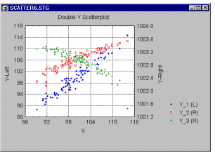
The Double-Y scatterplot can be used to compare images of several correlations by overlaying them in a single graph. However, due to the independent scaling used for the two list of variables, it can facilitate comparisons between variables with values in different ranges.
See also, Data Reduction.
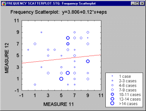
Scatterplot, 2D - Frequency. Frequency scatterplots display the frequencies of overlapping points between two variables in order to visually represent data point weight or other measurable characteristics of individual data points.
See also, Data Reduction.
Scatterplot, 2D - Multiple. Unlike the regular scatterplot in which one variable is represented by the horizontal axis and one by the vertical axis, the multiple scatterplot consists of multiple plots and represents multiple correlations: one variable (X) is represented by the horizontal axis, and several variables (Y's) are plotted against the vertical axis. A different point marker and color is used for each of the multiple Y-variables and referenced in the legend so that individual plots representing different variables can be discriminated in the graph.
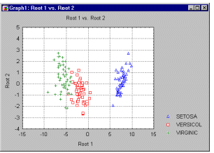
The Multiple scatterplot is used to compare images of several correlations by overlaying them in a single graph that uses one common set of scales (e.g., to reveal the underlying structure of factors or dimensions in Discriminant Function Analysis).
See also, Data Reduction.
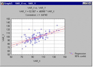
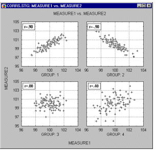
Scatterplot, 2D - Regular. The regular scatterplot visualizes a relation between two variables X and Y ( e.g., weight and height). Individual data points are represented by point markers in two- dimensional space, where axes represent the variables. The two coordinates (X and Y) which determine the location of each point, correspond to its specific values on the two variables. If the two variables are strongly related, then the data points form a systematic shape (e.g., a straight line or a clear curve). If the variables are not related, then the points form an irregular "cloud" (see the categorized scatterplot below for examples of both types of data sets).
Fitting functions to scatterplot data helps identify the patterns of relations between variables (see example below).
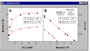
For more examples of how scatterplot data helps identify the patterns of relations between variables, see Outliers and Brushing. See also, Data Reduction.
Scatterplot, 3D. 3D Scatterplots visualize a relationship between three or more variables, representing the X, Y, and one or more Z (vertical) coordinates of each point in 3-dimensional space (see graph below).
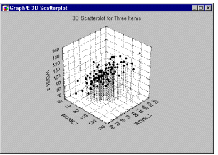
See also, 3D Scatterplot - Custom Ternary Graph, Data Reduction and Data Rotation (in 3D space).
Scatterplot, 3D - Raw Data. An unsmoothed surface (no smoothing function is applied) is drawn through the points in the 3D scatterplot.
See also, Data Reduction.Scatterplot, 3D - Ternary Graph. In this type of ternary graph, the triangular coordinate systems are used to plot four (or more) variables (the components X, Y, and Z, and the responses V1, V2, etc.) in three dimensions (ternary 3D scatterplots or surface plots). Here, the responses (V1, V2, etc.) associated with the proportions of the component variables (X, Y, and Z) in a ternary graph are plotted as the heights of the points.
See also, Data Reduction.
Scatterplot Smoothers. In 2D scatterplots, various smoothing methods are available to fit a function through the points to best represent (summarize) the relationship between the variables.
Scheffe's test. This post hoc test can be used to determine the significant differences between group means in an analysis of variance setting. Scheffe's test is considered to be one of the most conservative post hoc tests (for a detailed discussion of different post hoc tests, see Winer, Michels, & Brown (1991). For more details, see the General Linear Models chapter. See also, Post Hoc Comparisons. For a discussion of statistical significance, see Elementary Concepts.
Score Statistic. This statistic is used to evaluate the statistical significance of parameter estimates computed via maximum likelihood methods. It is also sometimes called the efficient score statistic. The test is based on the behavior of the log-likelihood function at the point where the respective parameter estimate is equal to 0.0 (zero); specifically, it uses the derivative (slope) of the log-likelihood function evaluated at the null hypothesis value of the parameter (parameter = 0.0). While this test is not as accurate as explicit likelihood-ratio test statistics based on the ratio of the likelihoods of the model that includes the parameter of interest, over the likelihood of the model that does not, its computation is usually much faster. It is therefore the preferred method for evaluating the statistical significance of parameter estimates in stepwise or best-subset model building methods.
An alternative statistic is the Wald statistic.
Scree Plot, Scree Test. The eigenvalues for successive factors can be displayed in a simple line plot. Cattell (1966) proposed that this scree plot can be used to graphically determine the optimal number of factors to retain.
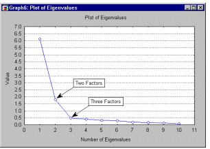
The scree test involves finding the place where the smooth decrease of eigenvalues appears to level off to the right of the plot. To the right of this point, presumably, one finds only "factorial scree" -- "scree" is the geological term referring to the debris which collects on the lower part of a rocky slope. Thus, no more than the number of factors to the left of this point should be retained.
For more information on procedures for determining the optimal number of factors to retain, see the section on Reviewing the Results of a Principal Components Analysis in the Factor Analysis chapter and How Many Dimensions to Specify in the Multi-dimensional Scaling chapter.
Semi-Partial (or Part) Correlation. The semi-partial or part correlation is similar to the partial correlation statistic. Like the, partial correlation, it is a measure of the correlation between two variables that remains after controlling for (i.e., "partialling" out) the effects of one or more other predictor variables. However, while the squared partial correlation between a predictor X1 and a response variable Y can be interpreted as the proportion of (unique) variance accounted for by X1, in the presence of other predictors X2, ... , Xk, relative to the residual or unexplained variance that cannot be accounted for by X2, ... , Xk, the squared semi-partial or part correlation is the proportion of (unique) variance accounted for by the predictor X1, relative to the total variance of Y. Thus, the semi-partial or part correlation is a better indicator of the "practical relevance" of a predictor, because it is scaled to (i.e., relative to) the total variability in the dependent (response) variable.
See also Correlation, Spurious Correlations, partial correlation, Basic Statistics, Multiple Regression, General Linear Models, General Stepwise Regression, Structural Equation Modeling (SEPATH).
SEMMA. See Models for Data Mining. See also Data Mining Techniques.
Sensitivity Analysis (in Neural Networks). A sensitivity analysis indicates which input variables are considered most important by that particular neural network. Sensitivity analysis can be used purely for informative purposes, or to perform input pruning.Sensitivity analysis can give important insights into the usefulness of individual variables. It often identifies variables that can be safely ignored in subsequent analyses, and key variables that must always be retained. However, it must be deployed with some care, for reasons that are explained below.
Input variables are not, in general, independent - that is, there are interdependencies between variables. Sensitivity analysis rates variables according to the deterioration in modeling performance that occurs if that variable is no longer available to the model. In so doing, it assigns a single rating value to each variable. However, the interdependence between variables means that no scheme of single ratings per variable can ever reflect the subtlety of the true situation.
Consider, for example, the case where two input variables encode the same information (they might even be copies of the same variable). A particular model might depend wholly on one, wholly on the other, or on some arbitrary combination of them. Then sensitivity analysis produces an arbitrary relative sensitivity to them. Moreover, if either is eliminated the model may compensate adequately because the other still provides the key information. It may therefore rate the variables as of low sensitivity, even though they might encode key information. Similarly, a variable that encodes relatively unimportant information, but is the only variable to do so, may have higher sensitivity than any number of variables that mutually encode more important information.
There may be interdependent variables that are useful only if included as a set. If the entire set is included in a model, they can be accorded significant sensitivity, but this does not reveal the interdependency. Worse, if only part of the interdependent set is included, their sensitivity will be zero, as they carry no discernable information.
In summary, sensitivity analysis does not rate the "usefulness" of variables in modeling in a reliable or absolute manner. You must be cautious in the conclusions you draw about the importance of variables. Nonetheless, in practice it is extremely useful. If a number of models are studied, it is often possible to identify key variables that are always of high sensitivity, others that are always of low sensitivity, and "ambiguous" variables that change ratings and probably carry mutually redundant information.
How does sensitivity analysis work? Each input variable is treated in turn as if it were "unavailable" (Hunter, 2000). There is a missing value substitution procedure, which is used to allow predictions to be made in the absence of values for one or more inputs. To define the sensitivity of a particular variable, v, we first run the network on a set of test cases, and accumulate the network error. We then run the network again using the same cases, but this time replacing the observed values of v with the value estimated by the missing value procedure, and again accumulate the network error.
Given that we have effectively removed some information that presumably the network uses (i.e. one of its input variables), we would reasonably expect some deterioration in error to occur. The basic measure of sensitivity is the ratio of the error with missing value substitution to the original error. The more sensitive the network is to a particular input, the greater the deterioration we can expect, and therefore the greater the ratio.
If the ratio is one or lower, then making the variable "unavailable" either has no effect on the performance of the network, or actually enhances it (!).
Once sensitivities have been calculated for all variables, they may be ranked in order.
Sequential Contour Plot, 3D. This contour plot presents a 2-dimensional projection of the spline-smoothed surface fit to the data (see 3D Sequential Surface Plot. Successive values of each series are plotted along the X-axis, with each successive series represented along the Y- axis.Sequential/Stacked Plots. In this type of graph, the sequence of values from each selected variable is stacked on one another.
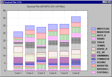
Sequential/Stacked Plots, 2D - Area. The sequence of values from each selected variable will be represented by consecutive areas stacked on one another in this type of graph.
Sequential/Stacked Plots, 2D - Column. The sequence of values from each selected variable will be represented by consecutive segments of vertical columns stacked on one another in this type of graph.
Sequential/Stacked Plots, 2D - Lines. The sequence of values from each selected variable will be represented by consecutive lines stacked on one another in this type of graph.
Sequential/Stacked Plots, 2D - Mixed Line. In this type of graph, the sequences of values of variables selected in the first list will be represented by consecutive areas stacked on one another while the sequences of values of variables selected in the second list will be represented by consecutive lines stacked on one another (over the area representing the last variable from the first list).
Sequential/Stacked Plots, 2D - Mixed Step. In this type of graph, the sequences of values of variables selected in the first list will be represented by consecutive step areas stacked on one another while the sequences of values of variables selected in the second list will be represented by consecutive step lines stacked on one another (over the step area representing the last variable from the first list).
Sequential/Stacked Plots, 2D - Step. The sequence of values from each selected variable will be represented by consecutive step lines stacked on one another in this type of graph.
Sequential/Stacked Plots, 2D - Step Area. The sequence of values from each selected variable will be represented by consecutive step areas stacked on one another in this type of graph.
Sequential Surface Plot, 3D. In this sequential plot, a spline-smoothed surface is fit to each data point. Successive values of each series are plotted along the X-axis, with each successive series represented along the Y-axis.
Sets of Samples in Quality Control Charts. While monitoring an ongoing process, it often becomes necessary to adjust the center line values or control limits, as those values are being refined over time. Also, one may want to compute the control limits and center line values from a set of samples that are known to be in control, and apply those values to all subsequent samples. Thus, each set is defined by a set of computation samples (from which various statistics are computed, e.g., sigma, means, etc.) and a set of application samples (to which the respective statistics, etc. are applied). Of course, the computation samples and application samples can be (and often are) not the same. To reiterate, you may want to estimate sigma from a set of samples that are known to be in control (the computation set), and use that estimate for establishing control limits for all remaining and new samples (the application set).
Note that each sample must be uniquely assigned to one application set; in other words, each sample has control limits based on statistics (e.g., sigma) computed for one particular set. The assignment of application samples to sets proceeds in a hierarchical manner, i.e., each sample is assigned to the first set where it "fits" (where the definition of the application sample set would include the respective sample). This hierarchical search always begins at the last set that the user specified, and not with the all-samples set. Hence, if the user-specified sets encompass all valid samples, the default all-samples set will actually become empty (since all samples will be assigned to one of the user-defined sets).
Shapiro-Wilks' W test. The Shapiro-Wilks' W test is used in testing for normality. If the W statistic is significant, then the hypothesis that the respective distribution is normal should be rejected. The Shapiro-Wilks' W test is the preferred test of normality because of its good power properties as compared to a wide range of alternative tests (Shapiro, Wilk, & Chen, 1968). Some software programs implement an extension to the test described by Royston (1982), which allows it to be applied to large samples (with up to 5000 observations). See also Kolmogorov-Smirnov test and Lilliefors test.
Shewhart Control Charts. This is a standard graphical tool widely used in statistical Quality Control. The general approach to quality control charting is straightforward: One extracts samples of a certain size from the ongoing production process. One then produces line charts of the variability in those samples, and consider their closeness to target specifications. If a trend emerges in those lines, or if samples fall outside pre-specified limits, then the process is declared to be out of control and the operator will take action to find the cause of the problem. These types of charts are sometimes also referred to as Shewhart control charts (named after W. A. Shewhart who is generally credited as being the first to introduce these methods; see Shewhart, 1931).
For additional information, see also Quality Control charts; Assignable causes and actions.
Short Run Control Charts. The short run quality control chart , for short production runs, plots transformations of the observations of variables or attributes for multiple parts, each of which constitutes a distinct "run," on the same chart. The transformations rescale the variable values of interest such that they are of comparable magnitudes across the different short production runs (or parts). The control limits computed for those transformed values can then be applied to determine if the production process is in control, to monitor continuing production, and to establish procedures for continuous quality improvement.
Shuffle data (in Neural Networks).Randomly assigning cases to the training and verification sets, so that these are (as far as possible) statistically unbiased. See, Neural Networks.
Shuffle, Back Propagation (in Neural Networks). Presenting training cases in a random order on each epoch, to prevent various undesirable effects which can otherwise occur (such as oscillation and convergence to local minima). See, Neural Networks.
Sigma Restricted Model. A sigma restricted model uses the sigma-restricted coding to represent effects for categorical predictor variables in general linear models and generalized linear models. To illustrate the sigma-restricted coding, suppose that a categorical predictor variable called Gender has two levels (i.e., male and female). Cases in the two groups would be assigned values of 1 or -1, respectively, on the coded predictor variable, so that if the regression coefficient for the variable is positive, the group coded as 1 on the predictor variable will have a higher predicted value (i.e., a higher group mean) on the dependent variable, and if the regression coefficient is negative, the group coded as -1 on the predictor variable will have a higher predicted value on the dependent variable. This coding strategy is aptly called the sigma-restricted parameterization, because the values used to represent group membership (1 and -1) sum to zero.
See also categorical predictor variables, design matrix; or General Linear Models.
Sigmoid function. An S-shaped curve, with a near-linear central response and saturating limits.
See also, logistic function and hyperbolic tangent function.
Signal detection theory (SDT). Signal detection theory (SDT) is an application of statistical decision theory used to detect a signal embedded in noise. SDT is used in psychophysical studies of detection, recognition, and discrimination, and in other areas such as medical research, weather forecasting, survey research, and marketing research.
A general approach to estimating the parameters of the signal detection model is via the use of the generalized linear model. For example, DeCarlo (1998) shows how signal detection models based on different underlying distributions can easily be considered by using the generalized linear model with different link functions.
For discussion of the generalized linear model and the link functions which it uses, see the Generalized Linear Models chapter.
Simple Random Sampling (SRS). Simple random sampling is a type of probability sampling where observations are randomly selected from a population with a known probability or sampling fraction. Typically, one begins with a list of N observations that comprises the entire population from which one wishes to extract a simple random sample (e.g., a list of registered voters); one can then generate k random case numbers (without replacement) in the range from 1 to N, and select the respective cases into the final sample (with a sampling fraction or known selection probability of k/N).
Refer to, for example, Kish (1965) for a detailed discussion of the advantages and characteristics of probability samples and EPSEM samples.
Simplex algorithm. A nonlinear estimation algorithm that does not rely on the computation or estimation of the derivatives of the loss function. Instead, at each iteration the function will be evaluated at m+1 points in the m dimensional parameter space. For example, in two dimensions (i.e., when there are two parameters to be estimated), the program will evaluate the function at three points around the current optimum. These three points would define a triangle; in more than two dimensions, the "figure" produced by these points is called a Simplex.Single and Multiple Censoring. There are situations in which censoring can occur at different times (multiple censoring), or only at a particular point in time (single censoring). Consider an example experiment where we start with 100 light bulbs, and terminate the experiment after a certain amount of time. If the experiment is terminated at a particular point in time, then a single point of censoring exists, and the data set is said to be single-censored. However, in biomedical research multiple censoring often exists, for example, when patients are discharged from a hospital after different amounts (times) of treatment, and the researcher knows that the patient survived up to those (differential) points of censoring.
Data sets with censored observations can be analyzed via Survival Analysis or via Weibull and Reliability/Failure Time Analysis. See also, Type I and II Censoring and Left and Right Censoring.
Singular Value Decomposition. An efficient algorithm for optimizing a linear model.
See also, pseudo-inverse.
![]() Six Sigma (DMAIC).
Six Sigma is a well-structured,
data-driven methodology for eliminating defects, waste, or quality control
problems of all kinds in manufacturing, service delivery, management,
and other business activities. Six Sigma
methodology is based on the combination of well-established statistical
quality control techniques, simple and advanced data analysis methods,
and the systematic training of all personnel at every level in the organization
involved in the activity or process targeted by Six
Sigma.
Six Sigma (DMAIC).
Six Sigma is a well-structured,
data-driven methodology for eliminating defects, waste, or quality control
problems of all kinds in manufacturing, service delivery, management,
and other business activities. Six Sigma
methodology is based on the combination of well-established statistical
quality control techniques, simple and advanced data analysis methods,
and the systematic training of all personnel at every level in the organization
involved in the activity or process targeted by Six
Sigma.
Six Sigma methodology and management strategies provide an overall framework for organizing company wide quality control efforts. These methods have recently become very popular, due to numerous success stories from major US-based as well as international corporations. For reviews of Six Sigma strategies, refer to Harry and Schroeder (2000), or Pyzdek (2001).
These are organized into the categories of activities that make up the Six Sigma effort: Define (D), Measure (M), Analyze (A), Improve (I), Control (C); or DMAIC for short.
Define. The Define phase is concerned with the definition of project goals and boundaries, and the identification of issues that need to be addressed to achieve the higher sigma level.
Measure. The goal of the Measure phase is to gather information about the current situation, to obtain baseline data on current process performance, and to identify problem areas.
Analyze. The goal of the Analyze phase is to identify the root cause(s) of quality problems, and to confirm those causes using the appropriate data analysis tools.
Improve. The goal of the Improve phase is to implement solutions that address the problems (root causes) identified during the previous (Analyze) phase.
Control. The goal of the Control phase is to evaluate and monitor the results of the previous phase (Improve).
Six Sigma Process. A six sigma process is one that can be expected to produce only 3.4 defects per one million opportunities. The concept of the six sigma process is important in Six Sigma quality improvement programs. The idea can best be summarized with the following graphs.
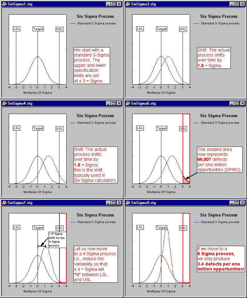
The term Six Sigma derives from the goal to achieve a process variation, so that ± 6 * sigma (the estimate of the population standard deviation) will "fit" inside the lower and upper specification limits for the process. In that case, even if the process mean shifts by 1.5 * sigma in one direction (e.g., to +1.5 sigma in the direction of the upper specification limit), then the process will still produce very few defects.
For example, suppose we expressed the area above the upper specification limit in terms of one million opportunities to produce defects. The 6 * sigma process shifted upwards by 1.5 * sigma will only produce 3.4 defects (i.e., "parts" or "cases" greater than the upper specification limit) per one million opportunities.
Shift. An ongoing process that at some point was centered will shift over time. Motorola, in their implementation of Six Sigma strategies, determined that it is reasonable to assume that a process will shift over time by approximately 1.5 * sigma (see, for example, Harry and Schroeder, 2000). Hence, most standard Six Sigma calculators will be based on a 1.5 * sigma shift.
One-sided vs. two-sided limits. In the illustration shown above the area outside the upper specification limit (greater than USL) is defined as one million opportunities to produce defects. Of course, in many cases any "outcomes" (e.g., parts) that are produced that fall below the specification limit can be equally defective. In that case one may want to consider the lower tail of the respective (shifted) normal distribution as well. However, in practice one usually ignores the lower tail of the normal curve because (1) in many cases, the process "naturally" has one-sided specification limits (e.g., very low delay times are not really a defect, only very long times; very few customer complaints are not a problem, only very many, etc.), and (2) when a 6 * sigma process has been achieved, the area under the normal curve below the lower specification limit is negligible.
Yield. The illustration shown above focuses on the number of defects that a process produces. The number of non-defects can be considered the Yield of the process. Six Sigma calculators will compute the number of defects per million opportunities (DPMO) as well as the yield, expressed as the percent of the area under the normal curve that falls below the upper specification limit (in the illustration above).
Skewness. Skewness (this term was first used by Pearson, 1895) measures the deviation of the distribution from symmetry. If the skewness is clearly different from 0, then that distribution is asymmetrical, while normal distributions are perfectly symmetrical.
Skewness = n*M3/[(n-1)*(n-2)* 3]
3]
where
M3 is equal to:  (xi-Meanx)3
 3 is the standard deviation (sigma) raised to the third power
n is the valid number of cases.
See also, Descriptive Statistics Overview.
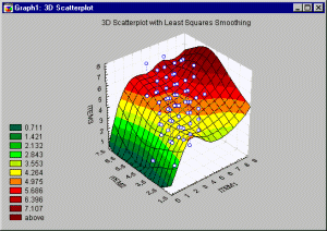
Smoothing. Smoothing techniques can be used in two different situations. Smoothing techniques for 3D Bivariate Histograms allow you to fit surfaces to 3D representations of bivariate frequency data. Thus, every 3D histogram can be turned into a smoothed surface providing a sensitive method for revealing non-salient overall patterns of data and/or identifying patterns to use in developing quantitative models of the investigated phenomenon.
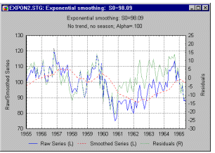
In Time Series analysis, the general purpose of smoothing techniques is to "bring out" the major patterns or trends in a time series, while de-emphasizing minor fluctuations (random noise). Visually, as a result of smoothing, a jagged line pattern should be transformed into a smooth curve.
See also, Exploratory Data Analysis and Data Mining Techniques, and Smoothing Bivariate Distributions.
SOFMs (Self-organizing feature maps; Kohonen Networks). Neural networks based on the topological properties of the human brain, also known as Kohonen Networks (Kohonen, 1982; Fausett, 1994,; Haykin, 1994; Patterson, 1996).
Softmax. A specialized activation function for one-of-N encoded classification networks. Performs a normalized exponential (i.e. the outputs add up to 1). In combination with the cross entropy error function, allows multilayer perceptron networks to be modified for class probability estimation (Bishop, 1995; Bridle, 1990). See, Neural Networks.
Space Plots. This type of graph offers a distinctive means of representing 3D Scatterplot data through the use of a separate X-Y plane positioned at a user-selectable level of the vertical Z-axis (which "sticks up" through the middle of the plane).
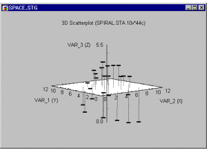
The Space Plots specific layout may facilitate exploratory examination of specific types of three-dimensional data. It is recommended to assign variables to axes such that the variable that is most likely to discriminate between patterns of relation among the other two is specified as Z.
See also, Data Rotation (in 3D space) in the Graphical Techniques chapter.
Spearman R. Spearman R can be thought of as the regular Pearson product-moment correlation coefficient (Pearson r); that is, in terms of the proportion of variability accounted for, except that Spearman R is computed from ranks. As mentioned above, Spearman R assumes that the variables under consideration were measured on at least an ordinal (rank order) scale; that is, the individual observations (cases) can be ranked into two ordered series. Detailed discussions of the Spearman R statistic, its power and efficiency can be found in Gibbons (1985), Hays (1981), McNemar (1969), Siegel (1956), Siegel and Castellan (1988), Kendall (1948), Olds (1949), or Hotelling and Pabst (1936).
Spectral Plot. The original application of this type of plot was in the context of spectral analysis in order to investigate the behavior of non-stationary time series. On the horizontal axes one can plot the frequency of the spectrum against consecutive time intervals, and indicate on the Z-axis the spectral densities at each interval (see for example, Shumway, 1988, page 82).
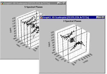
Spectral plots have clear advantages over the regular 3D Scatterplots when you are interested in examining how a relationship between two variables changes across the levels of a third variable, as is shown in the next illustration. The advantage of Spectral Plots over the regular 3D Scatterplots is well-illustrated in the comparison of the two displays of the same data set shown below.
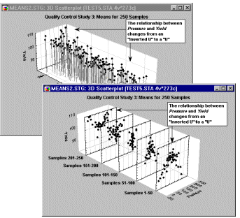
The Spectral Plot makes it easier to see that the relationship between Pressure and Yield changes from an "inverted U" to a "U".
See also, Data Rotation (in 3D space) in the Graphical Techniques chapter.
Spikes (3D graphs). In this type of graph, individual values of one or more series of data are represented along the X-axis as a series of "spikes" (point symbols with lines descending to the base plane). Each series to be plotted is spaced along the Y-axis. The "height" of each spike is determined by the respective value of each series.
Spline (2D graphs). A curve is fitted to the XY coordinate data using the bicubic spline smoothing procedure.
Spline (3D graphs). A surface is fitted to the XYZ coordinate data using the bicubic spline smoothing procedure.
Split Selection (for Classification Trees). Split selection for classification trees refers to the process of selecting the splits on the predictor variables which are used to predict membership in the classes of the dependent variable for the cases or objects in the analysis. Given the hierarchical nature of classification trees, these splits are selected one at time, starting with the split at the root node, and continuing with splits of resulting child nodes until splitting stops, and the child nodes which have not been split become terminal nodes.
The split selection process is described in the Computational Methods section of the Classification Trees chapter.
Spurious Correlations. Correlations that are due mostly to the influences of one or more "other" variables. For example, there is a correlation between the total amount of losses in a fire and the number of firemen that were putting out the fire; however, what this correlation does not indicate is that if you call fewer firemen then you would lower the losses. There is a third variable (the initial size of the fire) that influences both the amount of losses and the number of firemen. If you "control" for this variable (e.g., consider only fires of a fixed size), then the correlation will either disappear or perhaps even change its sign. The main problem with spurious correlations is that we typically do not know what the "hidden" agent is. However, in cases when we know where to look, we can use partial correlations that control for (i.e., partial out) the influence of specified variables.
See also Correlation, Partial Correlation, Basic Statistics, Multiple Regression, Structural Equation Modeling (SEPATH).
SQL.

For more information see the chapter on Power Analysis.
Stacked Generalization. See Stacking.
Stacking (Stacked Generalization). The concept of stacking (short for Stacked Generalization) applies to the area of predictive data mining, to combine the predictions from multiple models. It is particularly useful when the types of models included in the project are very different.Suppose your data mining project includes tree classifiers, such as C&RT and CHAID, linear discriminant analysis (e.g., see GDA), and Neural Networks. Each computes predicted classifications for a crossvalidation sample, from which overall goodness-of-fit statistics (e.g., misclassification rates) can be computed. Experience has shown that combining the predictions from multiple methods often yields more accurate predictions than can be derived from any one method (e.g., see Witten and Frank, 2000). In stacking, the predictions from different classifiers are used as input into a meta-learner, which attempts to combine the predictions to create a final best predicted classification. So, for example, the predicted classifications from the tree classifiers, linear model, and the neural network classifier(s) can be used as input variables into a neural network meta-classifier, which will attempt to "learn" from the data how to combine the predictions from the different models to yield maximum classification accuracy.
Other methods for combining the prediction from multiple models or methods (e.g., from multiple datasets used for learning) are Boosting and Bagging (Voting).
Standard Deviation. The standard deviation (this term was first used by Pearson, 1894) is a commonly-used measure of variation. The standard deviation of a population of values is computed as:
 = [
= [ (xi-µ)2/N]1/2
where
µ is the population mean
N is the population size.
The sample estimate of the population standard deviation is computed as:
s = [ (xi-x-bar)2/n-1]1/2
where
xbar is the sample mean
n is the sample size.
See also, Descriptive Statistics Overview.
Standard Error. The standard error (this term was first used by Yule, 1897) is the standard deviation of a mean and is computed as:std.err. = Ö(s2/n)
where
s2 is the sample variance
n is the sample size.
Standard Error of the Mean. The standard error of the mean (first used by Yule, 1897) is the theoretical standard deviation of all sample means of size n drawn from a population and depends on both the population variance (sigma) and the sample size (n) as indicated below:
 = (
= ( 2/n)1/2
where
 2 is the population variance and
n is the sample size.
Since the population variance is typically unknown, the best estimate for the standard error of the mean is then calculated as:
 = (s2/n)1/2
where
s2 is the sample variance (our best estimate of the population variance) and
n is the sample size.
See also, Descriptive Statistics Overview.
Standard Error of the Proportion. This
is the standard deviation of the distribution of the sample proportion
over repeated samples. If the population proportion is  , and the sample size is N, the standard error of the proportion when sampling from an infinite population is
sp = (p(1-p)/N)**1/2
For more information see the chapter on Power Analysis.
Standard residual value. This is the standardized residual value (observed minus predicted divided by the square root of the residual mean square).
See also, Mahalanobis distance, deleted residual and Cook’s distance.
Standardization.While in the everyday language, the term "standardization" means - converting to a common standard or making something conform to a standard (i.e., its meaning is similar to the term "normalization" in data analysis, see normalization), in statistics, this term has a very specific meaning and refers to the transformation of data by subtracting each value from some reference value (typically a sample mean) and diving it by the standard deviation (typically a sample SD). This important transformation will bring all values (regardless of their distributions and original units of measurement) to compatible units from a distribution with a mean of 0 and a standard deviation of 1. This transformation has a wide variety of applications because it makes the distributions of values easy to compare across variables and/or subsets. If applied to the input data, standardization also makes the results of a variety of statistical techniques entirely independent of the ranges of values or the units of measurements (see the discussion of these issues in Elementary Concepts, Basic Statistics, Multiple Regression, Factor Analysis, and others).
Standardized DFFITS. This is another measure of impact of the respective case on the regression equation. The formula for standardized DFFITS is
SDFITi = DFFITi/(si( i)1/2)
where hi is the leverage for the ith case
and
 i = 1/N + hi
See also, DFFITS, studentized residuals, and studentized deleted residuals. For more information see Hocking (1996) and Ryan (1997).
Standardized Effect (Es). A statistical effect expressed in convenient standardized units. For example, the standardized effect in a 2 Sample t-test is the difference between the two means, divided by the standard deviation, i.e.,
Es = (µ1 - µ2)/s
For more information see the chapter on Power Analysis.
Stationary Series (in Time Series). In Time Series analysis, a stationary series has a constant mean, variance, and autocorrelation through time (i.e., seasonal dependencies have been removed via Differencing).
Statistical Power. The probability of rejecting a false statistical null hypothesis.
For more information see the chapter on Power Analysis.
Statistical Process Control (SPC).The term Statistical Process Control (SPC) is typically used in context of manufacturing processes (although it may also pertain to services and other activities), and it denotes statistical methods used to monitor and improve the quality of the respective operations. By gathering information about the various stages of the process and performing statistical analysis on that information, the SPC engineer is able to take necessary action (often preventive) to ensure that the overall process stays in-control and to allow the product to meet all desired specifications. SPC involves monitoring processes, identifying problem areas, recommending methods to reduce variation and verifying that they work, optimizing the process, assessing the reliability of parts, and other analytic operations. SPC uses such basic statistical quality control methods as quality control charts (Sheward, Pareto, and others), capability analysis, gage repeatability/reproducibility analysis, and reliability analysis. However, also specialized experimental methods (DOE) and other advanced statistical techniques are often part of global SPC systems. Important components of effective, modern SPC systems are real-time access to data and facilities to document and respond to incoming QC data on-line, efficient central QC data warehousing, and groupware facilities allowing QC engineers to share data and reports (see also Enterprise SPC).
See also, Quality Control and Process Analysis.
For more information on process control systems, see the ASQC/AIAG's Fundamental statistical process control reference manual (1991).
Statistical Significance (p-level). The statistical significance of a result is an estimated measure of the degree to which it is "true" (in the sense of "representative of the population"). More technically, the value of the p-level represents a decreasing index of the reliability of a result. The higher the p-level, the less we can believe that the observed relation between variables in the sample is a reliable indicator of the relation between the respective variables in the population. Specifically, the p-level represents the probability of error that is involved in accepting our observed result as valid, that is, as "representative of the population." For example, the p-level of .05 (i.e.,1/20) indicates that there is a 5% probability that the relation between the variables found in our sample is a "fluke." In other words, assuming that in the population there was no relation between those variables whatsoever, and we were repeating experiments like ours one after another, we could expect that approximately in every 20 replications of the experiment there would be one in which the relation between the variables in question would be equal or stronger than in ours. In many areas of research, the p-level of .05 is customarily treated as a "border-line acceptable" error level.
See also, Elementary Concepts.
STATISTICA Advanced Linear/Nonlinear Models. StatSoft's STATISTICA Advanced Linear/Nonlinear Models offers a wide array of the most advanced modeling and forecasting tools on the market, including automatic model selection facilities and extensive interactive visualization tools.
 k+1 =
k+1 =  k +
k +  kgk
kgk
In simple terms, what this means is that the Hessian is not used to help find the direction for the next step. Instead, only the first derivative information in the gradient is used.
Hint for beginners. Inserting a few Steepest Descent Iterations may help in situations where the iterative routine "gets lost" after only a few iterations.
Stemming. An important pre-processing step before indexing input documents for text mining is the stemming of words. The term stemming refers to the reduction of words to their roots so that, for example, different grammatical forms or declinations of verbs are identified and indexed (counted) as the same word. For example, stemming will ensure that both "travel" and "traveled" will be recognized by the program as the same word.
For more information, see Manning and Schütze (2002).
Steps. Repetitions of a particular analytic or computational operation or procedure. For example in the neural network time series analysis, the number of consecutive time steps from which input variable values should be drawn to be fed into the neural network input units.
Stepwise Regression. A model-building technique which finds subsets of predictor variables that most adequately predict responses on a dependent variable by linear (or nonlinear) regression, given the specified criteria for adequacy of model fit.
For an overview of stepwise regression and model fit criteria see the General Stepwise Regression chapter, or the Multiple Regression chapter; for nonlinear stepwise and best subset regression, see the Generalized Linear Models chapter.
Stiffness Parameter (in Fitting Options). The function that controls the weight is determined by the Stiffness parameter which can be modified. Thus, the stiffness parameter determines the degree to which the fitted curve depends on local configurations of the analyzed values.
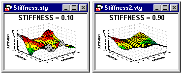
The lower the coefficient, the more the shape of the curve is influenced by individual data points (i.e., the curve "bends" more to accommodate individual values and subsets of values).
The range of the stiffness parameters is 0 < s < 1. Large values of the parameter produce smoother curves that adequately represent the overall pattern in the data set at the expense of local details.
See also, McLain, 1974.
Stopping Conditions. During an iterative process (e.g., fitting, searching, training), the conditions which must be true for the process to stop. (For example, in neural networks, the stopping conditions include the maximum number of epochs, target error performance and the minimum error improvement thresholds.
Stopping Conditions (in Neural Networks). The iterative gradient-descent training algorithms (back propagation, Quasi-Newton, conjugate gradient descent, Levenberg-Marquardt, quick propagation, Delta-bar-Delta, and Kohonen) all attempt to reduce the training error on each epoch.
You specify a maximum number of epochs for these iterative algorithms. However, you can also define stopping conditions that may cause training to determine earlier.
Specifically, training may be stopped when:
the error drops below a given level;
the error fails to improve by a given amount over a given number of epochs.
The conditions are cumulative; i.e., if several stopping conditions are specified, training ceases when any one of them is satisfied. In particular, a maximum number of epochs must always be specified.
The error-based stopping conditions can also be specified independently for the error on the training set and the error on the selection set (if any).
Target Error. You can specify a target error level, for the training subset, the selection subset, or both. If the RMS falls below this level, training ceases.
Minimum Improvement. Specifies that the RMS error on the training subset, the selection subset, or both must improve by at least this amount, or training will cease (if the Window parameter is non-zero).
Sometimes error improvement may slow down for a while or even rise temporarily (particularly if the shuffle option is used with back propagation, or non-zero noise is specified, as these both introduce an element of noise into the training process).
To prevent this option from aborting the run prematurely, specify a longer Window.
It is particularly recommended to monitor the selection error for minimum improvement, as this helps to prevent over-learning.
Specify a negative improvement threshold if you want to stop training only when a significant deterioration in the error is detected. The algorithm will stop when a number of generations pass during which the error is always the given amount worse than the best it ever achieved.
Window. The window factor is the number of epochs across which the error must fail to improve by the specified amount, before the algorithm is deemed to have slowed down too much and is stopped.
By default the window is zero, which means that the minimum improvement stopping condition is not used at all.
Stopping Rule (in Classification Trees). The stopping rule for a classification tree refers to the criteria that are used for determining the "right-sized" classification tree, that is, a classification tree with an appropriate number of splits and optimal predictive accuracy. The process of determining the "right-sized" classification tree is described in the Computational Methods section of the Classification Trees chapter.Stratified Random Sampling. In general, random sampling is the process of randomly selecting observations from a population, to create a subsample that "represents" the observations in that population (see Kish, 1965; see also Probability Sampling, Simple Random Sampling, EPSEM Samples; see also Representative Sample for a brief exploration of this often misunderstood notion). In stratified sampling one usually applies specific (identical or different) sampling fractions to different groups (strata) in the population to draw the sample.
Over-sampling particular strata to over-represent rare events. In some predictive data mining applications it is often necessary to apply stratified sampling to systematically over-sample (apply a greater sampling fraction) to particular "rare events" of interest. For example, in catalog retailing the response rate to particular catalog offers can be below 1%, and when analyzing historical data (from prior campaigns) to build a model for targeting potential customers more successfully, it is desirable to over-sample past respondents (i.e., the "rare" respondents who ordered from the catalog); one can then apply the various model building techniques for classification (see Data Mining) to a sample consisting of approximately 50% responders and 50% non-responders. Otherwise, if one were to draw a simple random sample for the analysis (with 1% of responders), then practically all model building techniques would likely predict a simple "no-response" for all cases, and would be (trivially) correct in 99% of the cases.
Stub and Banner Tables (Banner Tables). Stub-and-banner tables are essentially two-way tables, except that two lists of categorical variables (instead of just two individual variables) are crosstabulated. In the Stub-and-banner table, one list will be tabulated in the columns (horizontally) and the second list will be tabulated in the rows (vertically) of the Scrollsheet.For more information, see the Stub and Banner Tables section of the Basic Statistics chapter.
Student's t Distribution.
The Student's t distribution has density function (for  = 1, 2, ...):

where
 is the degrees of freedom
 (gamma) is the Gamma function
 is the constant Pi (3.14...)

The animation above shows various tail areas (p-values) for a Student's t distribution with 15 degrees of freedom.
Studentized Deleted Residuals. In addition to standardized residuals several methods (including studentized residuals, studentized deleted residuals, DFFITS, and standardized DFFITS) are available for detecting outlying values (observations with extreme values on the set of predictor variables or the dependent variable). The formula for studentized deleted residuals is given by
SDRESIDi = DRESIDi/ s(i)
for
DRESID = ei/(1- i )
i )
and where
s(i) = 1/(C-p-1)1/2 * ((C-p)s2/1-hi) - DRESIDi2)1/2
ei is the error for the ith case
hi is the leverage for the ith case
p is the number of coefficients in the model
and
 i = 1/N + hi
For more information see Hocking (1996) and Ryan (1997).
Studentized Residuals. In addition to standardized residuals several methods (including studentized residuals, studentized deleted residuals, DFFITS, and standardized DFFITS) are available for detecting outlying values (observations with extreme values on the set of predictor variables or the dependent variable). The formula for studentized residuals is
SRESi = (ei/s)/(1- i)1/2
i)1/2
where
ei is the error for the ith case
hi is the leverage for the ith case
and
 i = 1/N + hi
For more information see Hocking (1996) and Ryan (1997).
Sweeping. The sweeping transformation of matrices is commonly used to efficiently perform stepwise multiple regression (see Dempster, 1969, Jennrich, 1977) or similar analyses; a modified version of this transformation is also used to compute the g2 generalized inverse. The forward sweeping transformation for a column k can be summarized in the following four steps (where the e's refer to the elements of a symmetric matrix):
Sum-squared error function. An error function composed by squaring the difference between sets of target and actual values, and adding these together (see also, loss function.
Supervised and Unsupervised Learning. An important distinction in machine learning, and also applicable to data mining, is that between supervised and unsupervised learning algorithms. The term "supervised" learning is usually applied to cases in which a particular classification is already observed and recorded in a training sample, and you want to build a model to predict those classifications (in a new testing sample). For example, you may have a data set that contains information about who from among a list of customers targeted for a special promotion responded to that offer. The purpose of the classification analysis would be to build a model to predict who (from a different list of new potential customers) is likely to respond to the same (or a similar) offer in the future. You may want to review the methods discussed in General Classification and Regression Trees (GC&RT), General CHAID Models (GCHAID), Discriminant Function Analysis and General Discriminant Analysis (GDA), MARSplines (Multivariate Adaptive Regression Splines), and neural networks to learn about different techniques that can be used to build or fit models to data where the outcome variable of interest (e.g., customer did or did not respond to an offer) was observed. These methods are called supervised learning algorithms because the learning (fitting of models) is "guided" or "supervised" by the observed classifications recorded in the data file.
In unsupervised learning, the situation is different. Here the outcome variable of interest is not (and perhaps cannot be) directly observed. Instead, we want to detect some "structure" or clusters in the data that may not be trivially observable. For example, you may have a database of customers with various demographic indicators and variables potentially relevant to future purchasing behavior. Your goal would be to find market segments, i.e., groups of observations that are relatively similar to each other on certain variables; once identified, you could then determine how best to reach one or more clusters by providing certain goods or services you think may have some special utility or appeal to individuals in that segment (cluster). This type of task calls for an unsupervised learning algorithm, because learning (fitting of models) in this case cannot be guided by previously known classifications. Only after identifying certain clusters can you begin to assign labels, for example, based on subsequent research (e.g., after identifying one group of customers as "young risk takers").
There are several methods available for unsupervised learning, including Principal Components and Classification Analysis, Factor Analysis, Multidimensional Scaling, Correspondence Analysis, Neural Networks, Self-Organizing Feature Maps (SOFM, Kohonen networks); particularly powerful algorithms for pattern recognition and clustering are the EM and k-Means clustering algorithms.
Support Value (Association Rules). When applying (in data or text mining) algorithms for deriving association rules of the general form If Body then Head (e.g., If (Car=Porsche and Age<20) then (Risk=High and Insurance=High)), the Support value is computed as the joint probability (relative frequency of co-occurrence) of the Body and Head of each association rule.
Support Vector. A set of points in the feature space that determines the boundary between objects of different class memberships.
Support Vector Machine (SVM) Support Vector Machine (SVM) A classification method based on the maximum margin hyperplane.
Suppressor Variable. A suppressor variable (in Multiple Regression ) has zero (or close to zero) correlation with the criterion but is correlated with one or more of the predictor variables, and therefore, it will suppress irrelevant variance of independent variables. For example, you are trying to predict the times of runners in a 40 meter dash. Your predictors are Height and Weight of the runner. Now, assume that Height is not correlated with Time, but Weight is. Also assume that Weight and Height are correlated. If Height is a suppressor variable, then it will suppress, or control for, irrelevant variance (i.e., variance that is shared with the predictor and not the criterion), thus increasing the partial correlation. This can be viewed as ridding the analysis of noise.
Let t = Time, h = Height, w - Weight, rth = 0.0, rtw = 0.5, and rhw = 0.6.
Weight in this instance accounts for 25% (Rtw**2 = 0.5**2) of the variability of Time. However, if Height is included in the model, then an additional 14% of the variability of Time is accounted for even though Height is not correlated with Time (see below):
Rt.hw**2 = 0.5**2/(1 - 0.6**2) = 0.39
For more information, please refer to Pedhazur, 1982.
Surface Plot (from Raw Data). This sequential plot fits a spline-smoothed surface to each data point. Successive values of each series are plotted along the X-axis, with each successive series represented along the Y-axis.
Survival Analysis. Survival analysis (exploratory and hypothesis testing) techniques include descriptive methods for estimating the distribution of survival times from a sample, methods for comparing survival in two or more groups, and techniques for fitting linear or non-linear regression models to survival data. A defining characteristic of survival time data is that they usually include so-called censored observations, e.g., observations that "survived" to a certain point in time, and then dropped out from the study (e.g., patients who are discharged from a hospital). Instead of discarding such observations from the data analysis all together (i.e., unnecessarily loose potentially useful information) survival analysis techniques can accommodate censored observations, and "use" them in statistical significance testing and model fitting.Typical survival analysis methods include life table, survival distribution, and Kaplan-Meier survival function estimation, and additional techniques for comparing the survival in two or more groups. Finally, Survival analysis includes the use of regression models for estimating the relationship of (multiple) continuous variables to survival times.
For more information, see the Survival Analysis chapter.
Survivorship Function. The survivorship function (commonly denoted as R(t)) is the complement to the cumulative distribution function (i.e., R(t)=1-F(t)); the survivorship function is also referred to as the reliability or survival function (since it describes the probability of not failing or of surviving until a certain time t; e.g., see Lee, 1992).
For additional information see also the Survival Analysis chapter, or the Weibull and Reliability/Failure Time Analysis section in the Process Analysis chapter.
Symmetric Matrix. A matrix is symmetric if the transpose of the matrix is itself (i.e., A = A'). In other words, the lower triangle of the square matrix is a "mirror image" of the upper triangle with 1's on the diagonal (see below).
| |1 2 3 4| |2 1 5 6| |3 5 1 7| |4 6 7 1| |
Symmetrical Distribution. If you split the distribution in half at its mean (or median), then the distribution of values would be a "mirror image" about this central point.
See also, Descriptive Statistics Overview.
Synaptic Functions (in Neural Networks).Dot product. Dot product units perform a weighted sum of their inputs, minus the threshold value. In vector terminology, this is the dot product of the weight vector with the input vector, plus a bias value. Dot product units have equal output values along hyperplanes in pattern space. They attempt to perform classification by dividing pattern space into sections using intersecting hyperplanes.
Radial. Radial units calculate the square of the distance between the two points in N dimensional space (where N is the number of inputs) represented by the input pattern vector and the unit's weight vector. Radial units have equal output values lying on hyperspheres in pattern space. They attempt to perform classification by measuring the distance of normalized cases from exemplar points in pattern space (the exemplars being stored by the units). The squared distance is multiplied by the threshold (which is, therefore, actually a deviation value in radial units) to produce the post synaptic value of the unit (which is then passed to the unit's activation function).
Dot product units are used in multilayer perceptron and linear networks, and in the final layers of radial basis function, PNN, and GRNN networks.
Radial units are used in the second layer of Kohonen, radial basis function, Clustering, and probabilistic and generalized regression networks. They are not used in any other layers of any standard network architecture.
Division. This is specially designed for use in generalized regression networks, and should not be employed elsewhere. It expects one incoming weight to equal +1, one to equal -1, and the others to equal zero. The post-synaptic value is the +1 input divided by the -1 input.
